线性回归

1. 简介

线性回归是预测连续数值型变量的统计方法。它假设目标变量可以通过自变量（特征）的线性组合来近似表达。

单变量线性模型：

$$y=w_0+w_{1}x$$

多变量线性模型：

$$y=w_0+w_1{x}_1+w_2{x}_2+\dots +w_n{x}_n$$

其中 $w_0$ 为截距，$w_1,\dots ,w_n$ 为各特征的权重系数。

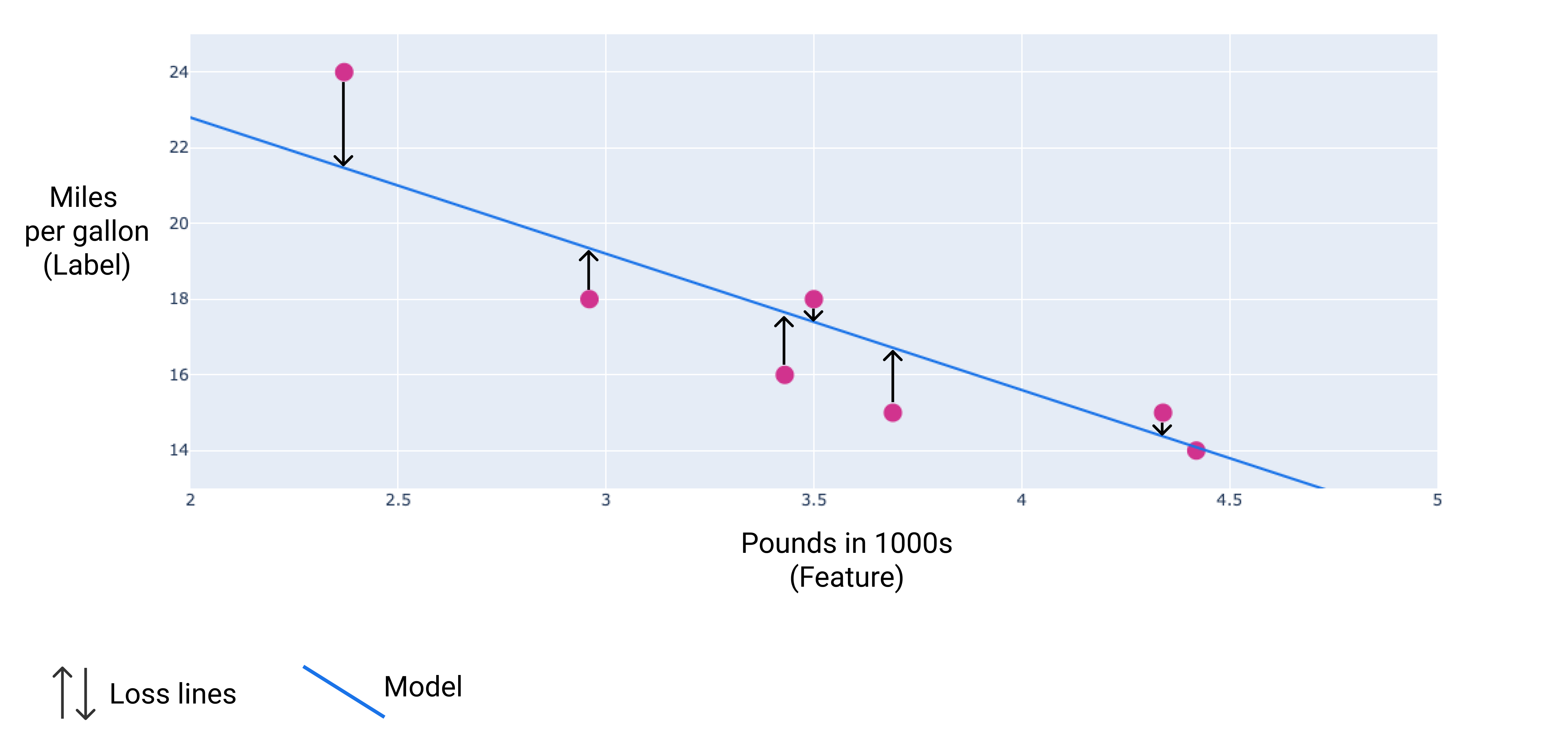
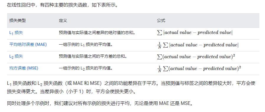
2. 损失函数

线性回归的目标是找到最优参数，使预测值与真实值的差异最小。

均方误差（MSE）：

$$\text{MSE}=\frac{1}{N}\sum _{i=1}^N{(y_i-{\hat{y}}_i)}^2$$

损失函数的几何理解

MSE 对应一个碗形（凸）曲面，梯度下降可以找到全局最小值。

3. 梯度下降求解

3.1 梯度推导

对损失函数关于参数 $w_j$ 求偏导：

$$\frac{\partial \text{MSE}}{\partial w_j}=-\frac{2}{N}\sum _{i=1}^N(y_i-{\hat{y}}_i)x_{ij}$$

3.2 参数更新

$$w_j\leftarrow w_j-\alpha \cdot \frac{\partial \text{MSE}}{\partial w_j}$$

3.3 向量化形式

$$\mathbf{w}\leftarrow \mathbf{w}-\frac{2\alpha }{N}{\mathbf{X}}^T(\mathbf{X}\mathbf{w}-\mathbf{y})$$

4. 解析解（正规方程）

对于线性回归，可以直接求得解析解：

$${\mathbf{w}}^{\ast }=({\mathbf{X}}^T\mathbf{X}{)}^{-1}{\mathbf{X}}^T\mathbf{y}$$

适用条件：特征数量较少（< 10000），且 $X^{T}X$ 可逆

5. 代码实现

5.1 从零实现

import numpy as np
import matplotlib.pyplot as plt

class LinearRegression:
    def __init__(self, lr=0.01, n_epochs=1000):
        self.lr = lr
        self.n_epochs = n_epochs
        self.weights = None
        self.bias = None
        
    def fit(self, X, y):
        m, n = X.shape
        self.weights = np.zeros(n)
        self.bias = 0
        
        losses = []
        for epoch in range(self.n_epochs):
            # 前向传播
            y_pred = X @ self.weights + self.bias
            
            # 计算损失
            loss = np.mean((y_pred - y) ** 2)
            losses.append(loss)
            
            # 计算梯度
            dw = (2/m) * X.T @ (y_pred - y)
            db = (2/m) * np.sum(y_pred - y)
            
            # 更新参数
            self.weights -= self.lr * dw
            self.bias -= self.lr * db
            
        return losses
    
    def predict(self, X):
        return X @ self.weights + self.bias

# 生成数据
np.random.seed(42)
m = 100
X = 2 * np.random.rand(m, 1)
y = 2 + 3 * X.ravel() + np.random.randn(m) * 0.5

# 训练
model = LinearRegression(lr=0.01, n_epochs=500)
losses = model.fit(X, y)
print(f"权重: {model.weights[0]:.3f}")   # 应接近 3
print(f"偏置: {model.bias:.3f}")         # 应接近 2

5.2 使用 scikit-learn

from sklearn.linear_model import LinearRegression
import numpy as np
import matplotlib.pyplot as plt

# 生成数据
np.random.seed(42)
m = 100
X = 2 * np.random.rand(m, 1)
y = 2 + 3 * X + np.random.randn(m, 1)

# 训练
lin_reg = LinearRegression()
lin_reg.fit(X, y)

print(f"截距：{lin_reg.intercept_[0]:.3f}")    # ≈ 2
print(f"斜率：{lin_reg.coef_[0][0]:.3f}")      # ≈ 3

# 预测
y_pred = lin_reg.predict(X)

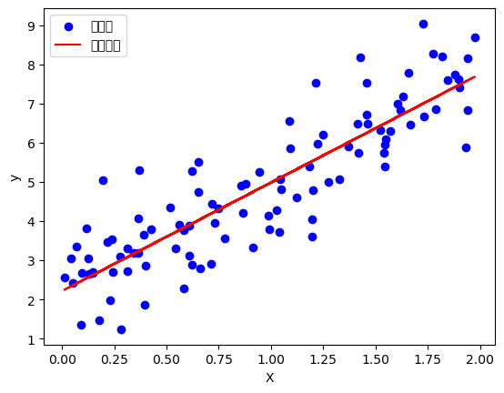
# 可视化
plt.figure(figsize=(8, 5))
plt.scatter(X, y, color="blue", alpha=0.5, label="数据点")
plt.plot(X, y_pred, color="red", linewidth=2, label="拟合直线")
plt.xlabel("X")
plt.ylabel("y")
plt.legend()
plt.title("线性回归")
plt.show()

6. 梯度 (Gradient) 详解

梯度是函数在某点沿各维度偏导数组成的向量：

$${\mathrm{\nabla }}_{\mathbf{w}}L=\left[\begin{array}{c}\frac{\partial L}{\partial w_1}\\ \frac{\partial L}{\partial w_2}\\ ⋮\\ \frac{\partial L}{\partial w_n}\end{array}\right]$$

对于 MSE 损失：

$${\mathrm{\nabla }}_{\mathbf{w}}L=\frac{2}{N}{\mathbf{X}}^T(\mathbf{X}\mathbf{w}-\mathbf{y})$$

def compute_gradient(X, y, w, b):
    """计算 MSE 损失的梯度"""
    m = len(y)
    y_pred = X @ w + b
    error = y_pred - y
    
    dw = (2/m) * X.T @ error
    db = (2/m) * np.sum(error)
    return dw, db

7. 学习率的影响

import numpy as np
import matplotlib.pyplot as plt

def gradient_descent_1d(lr, n_steps=30):
    """可视化不同学习率的梯度下降"""
    # f(w) = w^2，最小值在 w=0
    w = 5.0
    history = [w]
    
    for _ in range(n_steps):
        grad = 2 * w  # f'(w) = 2w
        w = w - lr * grad
        history.append(w)
    
    return history

fig, axes = plt.subplots(1, 3, figsize=(15, 4))
learning_rates = [0.1, 0.5, 1.1]
titles = ['合适的学习率 (α=0.1)', '大学习率 (α=0.5)', '过大学习率 (α=1.1)']

for ax, lr, title in zip(axes, learning_rates, titles):
    history = gradient_descent_1d(lr)
    ax.plot(history, 'b-o', markersize=4)
    ax.axhline(y=0, color='r', linestyle='--', label='最优解')
    ax.set_title(title)
    ax.set_xlabel('迭代次数')
    ax.set_ylabel('参数值 w')
    ax.legend()

plt.tight_layout()
plt.show()

8. 多元线性回归

import pandas as pd
from sklearn.linear_model import LinearRegression
from sklearn.model_selection import train_test_split
from sklearn.preprocessing import StandardScaler
from sklearn.metrics import mean_squared_error, r2_score
import numpy as np

# 波士顿房价数据（示例特征）
np.random.seed(42)
n = 1000
X = np.column_stack([
    np.random.randn(n) * 100 + 1500,  # 面积（㎡）
    np.random.randint(1, 6, n),        # 卧室数量
    np.random.randint(1, 50, n),       # 楼层
    np.random.randint(1990, 2024, n)   # 建成年份
])
y = 0.5 * X[:, 0] + 3000 * X[:, 1] - 200 * X[:, 2] + 100 * (X[:, 3] - 1990) + np.random.randn(n) * 10000

# 数据分割
X_train, X_test, y_train, y_test = train_test_split(X, y, test_size=0.2, random_state=42)

# 标准化
scaler = StandardScaler()
X_train_s = scaler.fit_transform(X_train)
X_test_s = scaler.transform(X_test)

# 训练
model = LinearRegression()
model.fit(X_train_s, y_train)

# 评估
y_pred = model.predict(X_test_s)
print(f"RMSE: {mean_squared_error(y_test, y_pred)**0.5:.2f}")
print(f"R²:   {r2_score(y_test, y_pred):.4f}")

9. 总结

特性	说明
任务类型	回归（连续值预测）
模型假设	特征与目标呈线性关系
优化方法	梯度下降 / 正规方程
损失函数	MSE（均方误差）
优点	简单、可解释、计算快
缺点	无法捕捉非线性关系
正则化版本	Ridge（L2）、Lasso（L1）、Elastic Net