LSTM（长短期记忆网络）

LSTM（Long Short-Term Memory）是 RNN 的关键升级版本，通过引入专用记忆通道（Cell State）和三个门控机制，解决了 RNN 的长距离依赖问题，成为 Transformer 出现前最强大的序列建模工具。

1. 为什么需要 LSTM？

RNN 的致命弱点：梯度消失导致无法记住远距离信息。

LSTM 的解决方案：引入两个状态 + 三个"门"：

RNN:  仅有 h_t（单一隐藏状态）
LSTM: h_t（短期记忆，对外输出）
      c_t（长期记忆，内部传输高速公路）

2. LSTM 结构总览

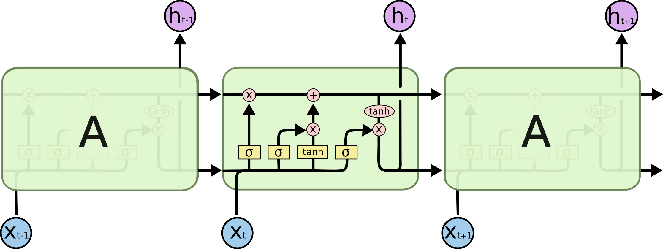
LSTM 在每个时间步维护两个状态：

• $h_t$：隐藏状态（短期记忆，对外输出）
• $c_t$：单元状态（长期记忆，内部高速公路）

核心创新：$c_t$ 通过加法更新而非乘法，梯度可以长距离无损传递！

3. 三个门控机制详解

遗忘门（Forget Gate）— 决定遗忘什么

$$f_t=\sigma (W_f\cdot [h_{t-1},x_t]+b_f)$$

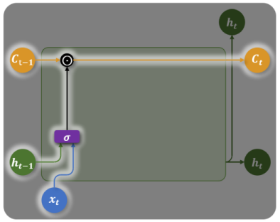
• 输入：当前输入 $x_t$ + 上一步隐藏状态 $h_{t-1}$
• 输出：$[0,1]$ 之间的向量（0=完全遗忘，1=完全保留）
• 乘以旧记忆 $c_{t-1}$，决定哪些历史信息要丢掉

比喻：读到新段落的第一句话，决定之前的主语信息是否还有用。

输入门（Input Gate）— 决定记住什么

$$i_t=\sigma (W_i\cdot [h_{t-1},x_t]+b_i)$$$${\tilde{c}}_t=\tanh (W_c\cdot [h_{t-1},x_t]+b_c)$$$$c_t=f_t\odot c_{t-1}+i_t\odot {\tilde{c}}_t$$

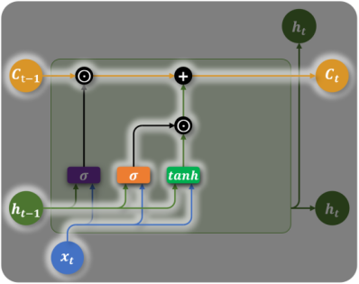
• $i_t$：控制当前信息的写入比例
• ${\tilde{c}}_t$：候选记忆（当前时间步提取的新信息）
• 单元状态更新：旧记忆（遗忘后）+ 新信息（写入后）

关键：$c_t$ 通过加法更新，梯度不消失！

输出门（Output Gate）— 决定输出什么

$$o_t=\sigma (W_o\cdot [h_{t-1},x_t]+b_o)$$$$h_t=o_t\odot \tanh (c_t)$$

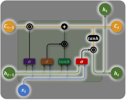
• $o_t$：控制记忆单元中哪些信息对外输出
• 对 $c_t$ 压缩到 $(-1,1)$ 再过滤输出

4. 完整公式汇总

门控	公式	作用
遗忘门	$f_t=\sigma (W_f[h_{t-1},x_t]+b_f)$	决定遗忘旧记忆的比例
输入门	$i_t=\sigma (W_i[h_{t-1},x_t]+b_i)$	决定写入新记忆的比例
候选记忆	${\tilde{c}}_t=\tanh (W_c[h_{t-1},x_t]+b_c)$	当前时间步的候选新信息
记忆更新	$c_t=f_t\odot c_{t-1}+i_t\odot {\tilde{c}}_t$	加法更新（关键！）
输出门	$o_t=\sigma (W_o[h_{t-1},x_t]+b_o)$	决定当前对外输出的内容
隐藏状态	$h_t=o_t\odot \tanh (c_t)$	对外输出的短期记忆

5. 变量维度

变量	维度	含义
$x$	[batch, seq_len, input_dim]	输入序列
$h_t$	[batch, hidden_dim]	每步隐藏状态（对外输出）
$c_t$	[batch, hidden_dim]	每步单元状态（内部长期记忆）
$f_t,i_t,o_t,{\tilde{c}}_t$	[batch, hidden_dim]	各门控输出

6. PyTorch 实现

基础使用

import torch
import torch.nn as nn

class LSTMModel(nn.Module):
    def __init__(self, input_dim, hidden_dim, output_dim, num_layers=1):
        super().__init__()
        self.lstm = nn.LSTM(
            input_size=input_dim,
            hidden_size=hidden_dim,
            num_layers=num_layers,
            batch_first=True,
            dropout=0.3 if num_layers > 1 else 0,
            bidirectional=False   # 单向 LSTM
        )
        self.fc = nn.Linear(hidden_dim, output_dim)
        self.dropout = nn.Dropout(0.3)
    
    def forward(self, x):
        # output: [batch, seq_len, hidden_dim]
        # h_n:    [num_layers, batch, hidden_dim]
        # c_n:    [num_layers, batch, hidden_dim]
        output, (h_n, c_n) = self.lstm(x)
        
        # 取最后一个时间步用于分类
        last_output = output[:, -1, :]        # [batch, hidden_dim]
        return self.fc(self.dropout(last_output))

# 使用
model = LSTMModel(input_dim=100, hidden_dim=256, output_dim=2)
x = torch.randn(32, 20, 100)   # [batch=32, seq_len=20, input=100]
out = model(x)
print(out.shape)                # [32, 2]

双向 LSTM（Bidirectional LSTM）

双向 LSTM 同时从正向和反向处理序列，捕获更完整的上下文：

class BiLSTMClassifier(nn.Module):
    def __init__(self, vocab_size, embed_dim, hidden_dim, output_dim):
        super().__init__()
        self.embedding = nn.Embedding(vocab_size, embed_dim)
        self.lstm = nn.LSTM(
            embed_dim, hidden_dim,
            batch_first=True, bidirectional=True  # 双向
        )
        # 双向输出拼接，维度 * 2
        self.fc = nn.Linear(hidden_dim * 2, output_dim)
        self.dropout = nn.Dropout(0.3)
    
    def forward(self, x):
        embedded = self.dropout(self.embedding(x))   # [batch, seq, embed]
        output, (h_n, c_n) = self.lstm(embedded)
        
        # 拼接正向最后 + 反向最后的隐藏状态
        # h_n: [2, batch, hidden]（2 = 双向）
        h_forward  = h_n[0, :, :]   # 正向最后时间步
        h_backward = h_n[1, :, :]   # 反向最后时间步
        h_cat = torch.cat([h_forward, h_backward], dim=1)   # [batch, hidden*2]
        
        return self.fc(self.dropout(h_cat))

model = BiLSTMClassifier(vocab_size=10000, embed_dim=128, 
                         hidden_dim=256, output_dim=3)

多层堆叠 LSTM

# 2 层 LSTM，隐藏层之间加 Dropout
lstm = nn.LSTM(
    input_size=100,
    hidden_size=256,
    num_layers=2,       # 堆叠层数
    batch_first=True,
    dropout=0.3         # 层间 Dropout
)

7. LSTM 的局限性

三大核心缺陷

缺陷	原因	Transformer 的改进
无法并行	$h_t$ 依赖 $h_{t-1}$，必须串行计算	自注意力：全序列并行
仍有长距离遗忘	100+ 步后仍有信息衰减	Attention 直接建模任意两点关系
计算复杂	每步 4 个全连接（4× RNN 参数量）	虽然参数多但可并行化

"LSTM 是设计精巧的蒸汽机，Transformer 是新时代的电力引擎。"

何时还使用 LSTM？

• 实时推理（Transformer 计算延迟高）
• 资源受限的边缘设备
• 短序列任务（< 200 步）
• 时间序列预测（不需要预训练的场景）

8. RNN vs LSTM vs Transformer

对比	RNN	LSTM	Transformer
状态	$h_t$	$h_t+c_t$（双状态）	无序列状态（全局注意力）
长依赖	差	中等（<100步）	强（任意长度）
并行性	❌	❌	✅
梯度消失	严重	缓解	无问题
主流地位	已基本淘汰	特定场景使用	当前主流

总结

特性	LSTM
提出时间	1997（Hochreiter & Schmidhuber）
核心创新	Cell State + 三门控（遗忘/输入/输出）
关键优势	加法更新记忆，解决梯度消失
主要弱点	无法并行，长序列仍有遗忘
典型应用	机器翻译（Pre-Transformer时代），时序预测